Exporting Transactions from a Chase Bank Account to Import (Load) into the Excel Checkbook Register

If you have bank accounts with Chase, here are the steps to get your bank transactions into the Excel Checkbook. It’s best if you already have some comfort with Microsoft Excel including the entry of basic formulas. You can follow these steps every time you want to get your bank transactions. Or maybe you want to get the previous year’s transactions? In either case, we’ll start with a summary.

Summary

• Export your transactions from the Chase website to a CSV file format
• Open that CSV file using Microsoft Excel, and reformat the data so that it has a similar column layout as the Excel checkbook template. This step includes the need to put deposits and withdrawals into a separate column since Chase puts all amounts in one column.
• Open the Excel Checkbook template and set the opening balance in cell G6 (if this is your first time using the Excel Checkbook)
• Copy transactions from the Chase CSV file and paste them into the checkbook template, starting in cell A7 (if this is your first time). If you have existing transactions, paste them after the last entries that you already have.
• (Optional) Review each transaction and specify a sub-category for each so that the Dashboard can properly show your income and expenses by category.

Exporting Transactions from Chase

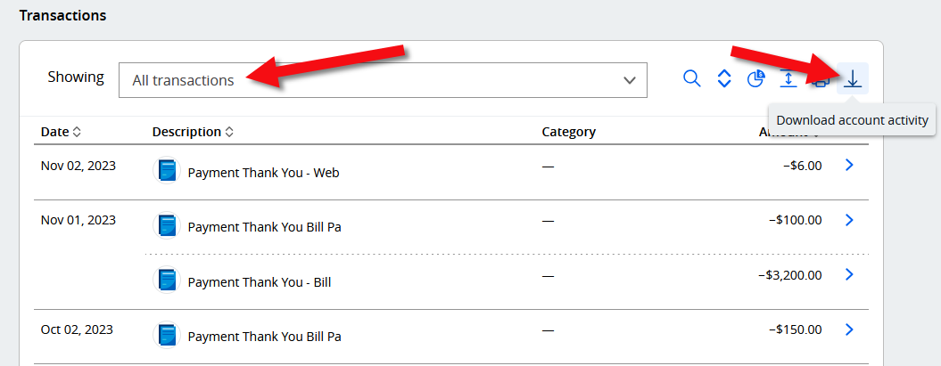
After logging into the Chase website, click on your account to see current transactions. There’s a button for Download account activity to get your transactions (see red arrows below). In the box labeled “Showing”, you can specify a date range or pick “All transactions”.

On the screen that follows, the file type will default to “Spreadsheet (Excel, CSV)”, which is what we want. Click Download.

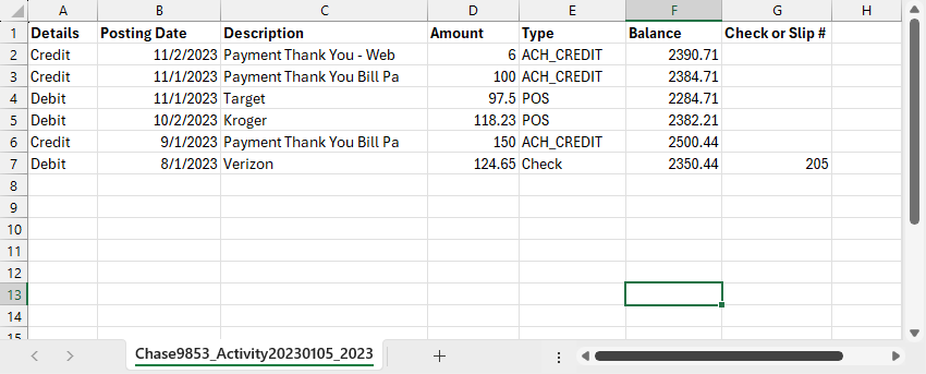
After download, you can open the file in Microsoft Excel. Your result should be similar to the sample screenshot below. Note: this sample has already been reformatted for easier readability in that the columns were widened and the top row was made bold. Doing so is not required.

Reformatting Steps to Take

• Cut and paste the Details column (column A) and move it to be before the Balance column. To do so, right-click on the “A” column and choose Cut. Then right-click on the “F” column and choose Insert Cut Cells.
• Cut and paste the Type column (column D) and move it before the Description column. Use the technique described in the previous step to do so.
• Cut and paste the Check column (column G) and move it before the Description column.
• Insert a new column before Amount, and call it Withdrawal
• Insert another new column before Amount, and call it Deposit

When you’re done, your spreadsheet should look something like this:

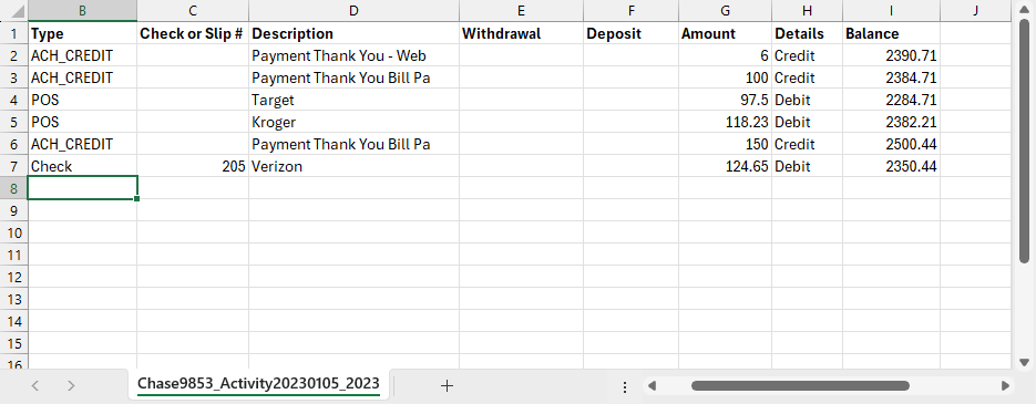
If your spreadsheet looks like the sample above with the Withdrawal column in “E”, enter the following formula into the E2 cell:

=IF(H2="Debit",G2,"")

After doing so, copy that formula all the way down the sheet. The quickest way to do so is by pointing your mouse on cell E2 but at the bottom-right corner until you see a black plus symbol. Then double-click.

Enter this formula into the F2 cell:

=IF(H2="Credit",G2,"")

Copy that formula down the sheet just like you did for the E2 formula.

At this point, your spreadsheet should look something like this:

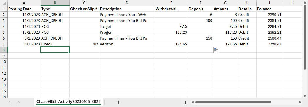
You are now ready to copy & paste your transactions from this CSV file into your Excel Checkbook register. Be sure to use “Paste as Values” when you paste into the Excel Checkbook register. See this video for a helpful guide on copying & pasting transactions. You can skip ahead to the 2:55 minute mark. The following video was made to show how to copy data between an older spreadsheet and a newer checkbook spreadsheet, but the copy/paste process that you’ll need to follow is identical.