If you have bank accounts with USAA, here are the steps to get your bank transactions into the Excel Checkbook. It’s best if you already have some comfort with Microsoft Excel including the entry of basic formulas. You can follow these steps every time you want to get your bank transactions. Or maybe you want to get the previous year’s transactions? In either case, we’ll start with a summary.
Summary
- Export your transactions from the USAA website to a CSV file format
- Open that CSV file using Microsoft Excel, and reformat the data so that it has a similar column layout as the Excel checkbook template. This step includes the need to put deposits and withdrawals into a separate column since USAA puts all amounts in one column.
- Open the Excel Checkbook template and set the opening balance in the first row (if this is your first time using the Excel Checkbook)
- Copy transactions from the CSV file and paste them into the checkbook template, starting in the row that immediately follows the starting balance (e.g., cell A8), or after any existing transactions that you have already added to the register.
- (Optional) Review each transaction and specify a sub-category for each so that the Dashboard can properly show your income and expenses by category.
Note: the steps that follow are an excellent candidate for a recorded macro. By recording a macro for this, you can quickly download recent bank transactions; run your macro; and the transactions are now ready for a quick copy/paste into your checkbook. See this YouTube video for an example of recording an Excel macro.
Exporting Transactions from USAA
After logging into the USAA website, Click on the name of the account for which you want to download transactions. Find the export/download option which is usually via the “I want to” menu in the upper-left corner and select “Export”. Alternatively, search for a “Summary” or “Transaction History” page and look for an “Export” or “Download” button.
Choose the Comma-Delimited (CSV) file type from the drop-down list. Choose the date range (if applicable): Use the filters on the transaction history page to select the specific period you need, if a direct download of a custom range isn’t an option.
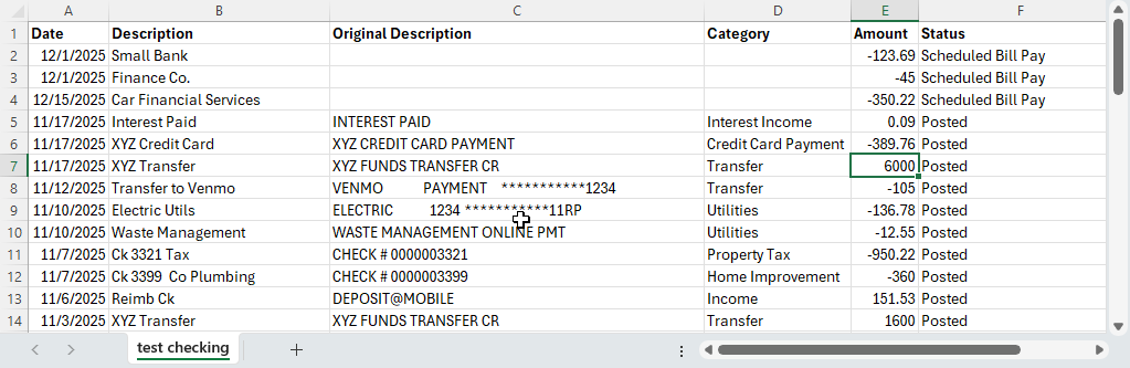
After download, you can open the file in Microsoft Excel. Your result should be similar to the sample screenshot below. Note: this sample has already been reformatted for easier readability in that the columns were widened and the top row was made bold. Doing so is not required.
Next Steps
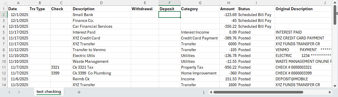
- Since the file has two columns for description, we’ll use the cleaner/easier to read description, and we’ll move the “Original Description” to the far right. Note: the column called “Original Description” will be needed in order to extract the check number when it’s a check transaction. Right-click on the “C” column (original description); choose Cut; right-click on the “G” column, and choose Insert Cut Cells.
- Insert two new columns after the Date column by right-clicking on the “B” column, then choose Insert. Do this twice. For the first new column (B), let’s name it Trx Type, and name the 3rd column (C) as Check.
- Paste the following formula into cell C2:
=IF(LEFT(H2,7)="CHECK #", VALUETOTEXT(VALUE(MID(H2, FIND("# ",H2)+2, 99))), "")Note: the formula above uses VALUETOTEXT which is a function that is not available in versions of Excel before 2021. As an alternative for older versions of Excel, you can try:
=IF(LEFT(H2,7)=”CHECK #”, VALUE(MID(H2, FIND(“# “,H2)+2, 99)), “”)
- After doing so, copy that formula all the way down the sheet. The quickest way to do so is by pointing your mouse on cell C2 but point at the bottom-right corner until you see a black plus symbol. Then double-click.
- Insert a new column before Category, and call it Withdrawal
- Insert another new column before Amount, and call it Deposit
When you’re done, your spreadsheet should look something like this:
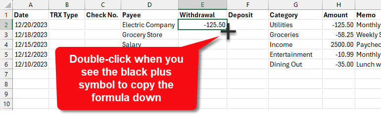
If your spreadsheet looks like the sample above with the Withdrawal column in “E”, enter the following formula into the E2 cell:
=IF(H2<0,H2*-1,0)After doing so, copy that formula all the way down the sheet. The quickest way to do so is by pointing your mouse on cell E2 but at the bottom-right corner until you see a black plus symbol. Then double-click.
Enter this formula into the F2 cell:
=IF(H2>0,H2,0)Copy that formula down the sheet just like you did for the E2 formula.
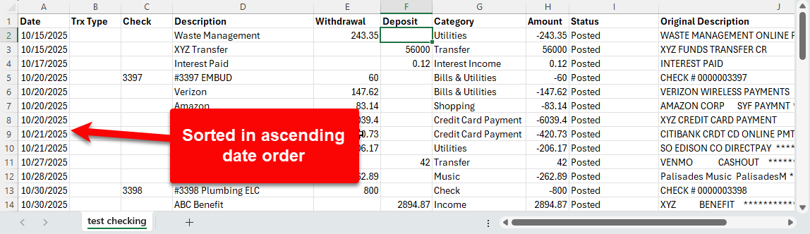
The last step will be to sort the transactions in ascending date order (oldest to newest).
After doing so, your spreadsheet should look something like this:
You are now ready to copy & paste your transactions from this CSV file into your Excel Checkbook register. Be sure to use “Paste as Values” when you paste into the Excel Checkbook register. Select the cells, starting with A2 (the first date) and include the columns of A – F, but don’t select beyond the Deposit column.
With your cells selected, you can now copy that to your clipboard by either pressing Ctrl+C (for Windows), or Command+C (for Mac), or right-click and choose Copy. Then switch to your Excel checkbook spreadsheet, find an empty row at the bottom, and use paste as values which is available as a right-click option.
NOTE: it is super important that you use paste as values when pasting to the Excel Checkbook. Don’t use “Paste Values & Source Formatting” and don’t use “Paste Values & Number Formatting” and don’t use just regular “Paste”. Those options will result in issues! So it has to be the plain-ole “Paste as Values”.
See this video for a helpful guide on copying & pasting transactions. You can skip ahead to the 2:55 minute mark. The following video was made to show how to copy data between an older spreadsheet and a newer checkbook spreadsheet, but the copy/paste process that you’ll need to follow is identical.
Discover more from Excel Checkbook
Subscribe to get the latest posts sent to your email.