Exporting Data from Quicken to Import (Load) into the Excel Checkbook Register

If you are moving from Quicken to the Excel Checkbook and you’d like to bring your existing data from Quicken, here are the steps. It’s best if you already have some comfort with Excel and entering basic formulas. We’ll start with a summary.

Summary

• Export your transactions from Quicken to a CSV file format or Tab-delimited format
• Open that text file using Microsoft Excel (via the Data menu –> From Text), and reformat the data so that it has a similar column layout as the Excel checkbook template. This step includes the need to put deposits into a separate column since Quicken puts all amounts in one column.
• Open the Excel Checkbook template and input your opening balance in the first row under the Deposit column.
• Copy transactions from the Quicken export and paste them into the checkbook template, starting in the row that immediately follows your starting balance
• Copy the category values from the Quicken export and paste them into the checkbook template under the Sub-Category column
• Review the category values and update them as needed to match with prior Quicken categories

Exporting Transactions from Quicken

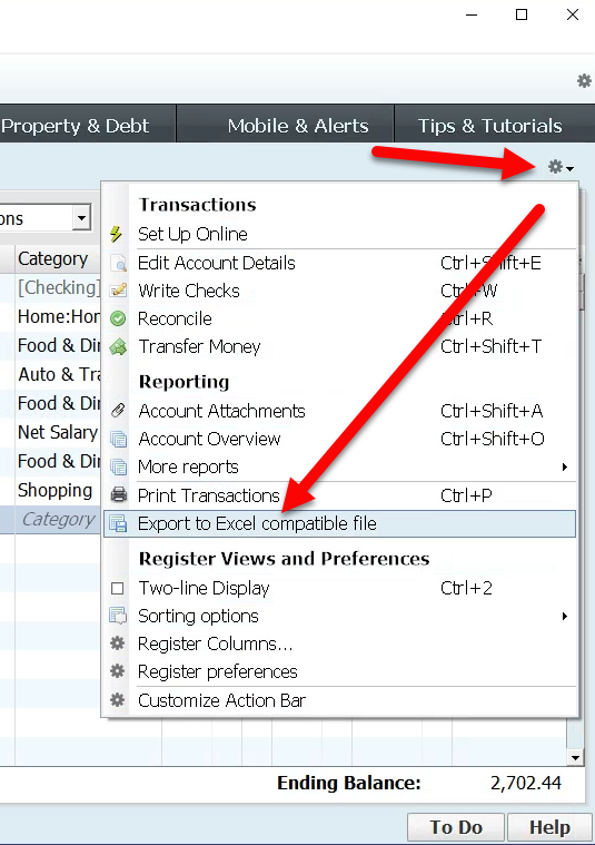
According to online posts, the way to export your transaction data is to be in the account register, and then select the PRINT function (or the cog-wheel) and select “Export To” and select the “tab delimited” option. Other online help articles say that you can export your data by visiting the Quicken report that shows your transactions, and then click the button for Export Data. Please note that Quicken displays the Export Data button only for reports, not graphs.

Here’s how the export option looks in an earlier version of Quicken:

After saving your data to a tab-delimited file, you should open it in Excel in the following manner.

• Open Microsoft Excel and go to a new (blank) workbook
• Visit the Data menu and choose From Text/CSV

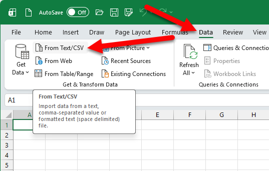
• Navigate in your folders to find your Quicken export file and choose it
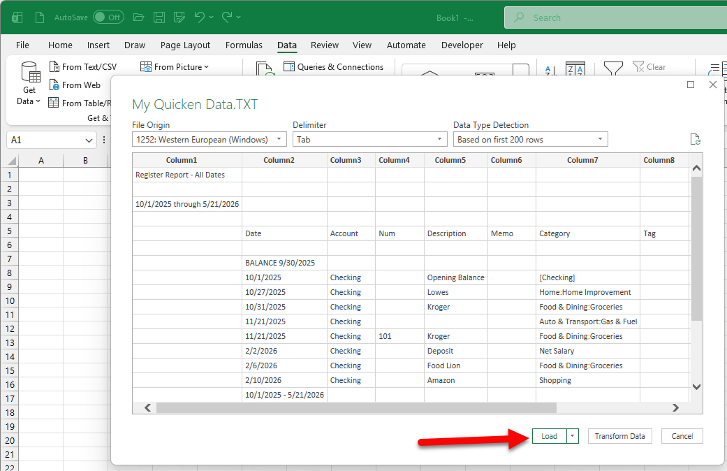
• Depending on your version of Microsoft Excel, the next screen will vary. In newer versions of Excel, it will look like the following where a preview of your data is displayed and Excel will automatically determine that a “Tab” is the special delimiter between each column of data. Click the Load button to finish opening the Quicken export.

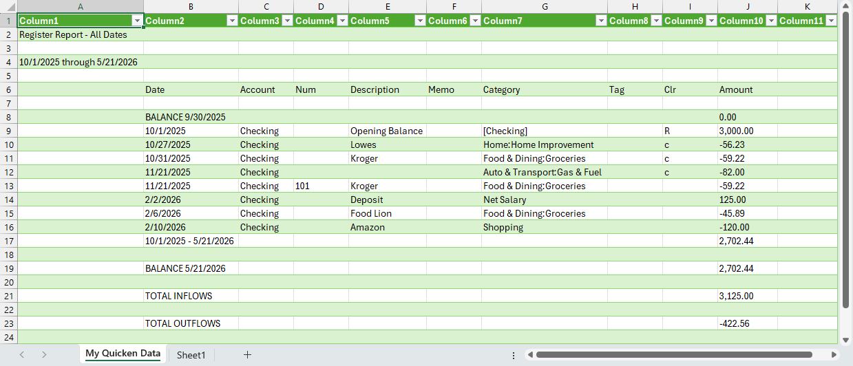
Here’s an example of what it might look like after clicking the “Load” button.

Reformatting Steps – See video at bottom of page for examples of these steps

• [Optional] Consider deleting the first column (column isn’t needed)
• [Optional] Copy the headings (Date, Account, Num, etc.) to the very top of the table
• [Optional] Delete the blank rows that appear above your transactions
• Move the Account column to the far right, after the Amount column. To do so, right-click that “B” column and choose “Cut”, and then right-click on the “J” column and choose “Insert Cut Cells”. (Note: column letters mentioned above assume you deleted the first column).
• Move the Memo and Category columns to the far right, perhaps to be located between Amount and Account (placement is not critical)
• Insert a new column between Date and Num and call it TRX Type.
• Insert a new column after Description and call it Withdrawal
• Insert a new column after Withdrawal and call it Deposit

When you’re done, your spreadsheet should look something like this:

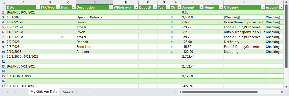
If your spreadsheet looks like the sample above with the Withdrawal column in “E” and the Amount column in “I”, enter the following formula into the E2 cell.

=IF(VALUE(I3)<0, VALUE(I3)*-1, 0)

About the formula: the “VALUE” function converts any numbers that Excel might have formatted as “text” to be actual numbers. Adjust the column letter references if your withdrawal or amount columns are in different lettered columns.

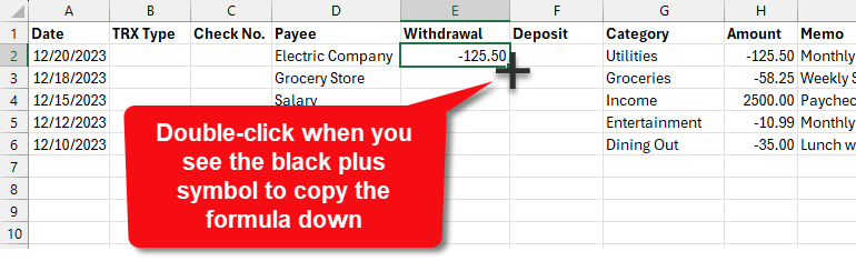
After doing so, you might have to copy that formula all the way down the sheet. However, if your screen has the alternating row colors like the example above, the formula will likely auto-fill down the worksheet. If not, the quickest way to copy the formula is by pointing your mouse on cell E2 but at the bottom-right corner until you see a black plus symbol. Then double-click.

Enter this formula into the F2 cell:

=IF(VALUE(I2)>0, VALUE(I2), 0)

Only if needed, copy that formula down the sheet just like you did for the previous formula.

At this point, your spreadsheet should look something like this:

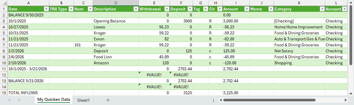
Note: if you see #VALUE errors in any cells, you can usually disregard since those are rows that didn’t have an amount for the formula to reference.

Before moving on, if your Quicken export has multiple accounts in your spreadsheet, I recommend that you sort your spreadsheet on the Account column since you’ll probably want to copy the transactions for each account into different register worksheets in the Excel Checkbook. Also, depending on how many years of data you have, you might want to consider only copying the last few years of transactions to the Excel Checkbook. While Microsoft Excel can easily handle 10’s of thousands of rows of transactions, for performance reasons, I recommend only copying the last 3 – 5 years of Quicken transactions to the checkbook.

You should now be ready to copy & paste your transactions from this Quicken file into your Excel Checkbook register. Be sure to use “Paste as Values” when you paste into the Excel Checkbook register.

NOTE: it is super important that you use paste as values when pasting to the Excel Checkbook. Don’t use “Paste Values & Source Formatting” and don’t use “Paste Values & Number Formatting” and don’t use just regular “Paste”. Those options will result in issues! So it has to be the plain-ole “Paste as Values”.

See this video for a helpful guide on copying & pasting transactions.